A story about value at risk
How would you define risk if you have a portfolio with a variety of assets? The Value at Risk (VaR) became popular in the early '90s through a publication by JP Morgan. They eased their quantitative market analysis with this comprehensive method. Due to the VaR it was no longer necessary to regularly work through a cumbersome process based on absolute market risk limits. Now they were able to set a limit based on probability.
VaR = μ + Z × σ
where:
- μ represents the mean of the returns,
- Z represents the Z-score corresponding to the confidence level (assuming a normal distribution). The z-score should be negative if you want to determine the left side of the mean,
- σ represents the standard deviation of the returns.
The Value at Risk parameter determines the market risk of a portfolio, meaning the risk of the portfolio related to historical average return and its standard deviation. It was created to hedge a portfolio while including diversification effects. This is done by considering the covariance of the assets in the portfolio. The basic idea here is to hedge/mitigate any dependencies the assests have. It calculates the impact of systematic risk on your portfolio.
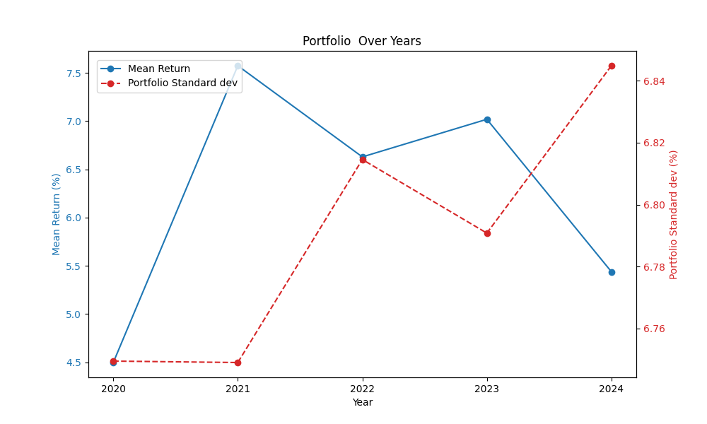
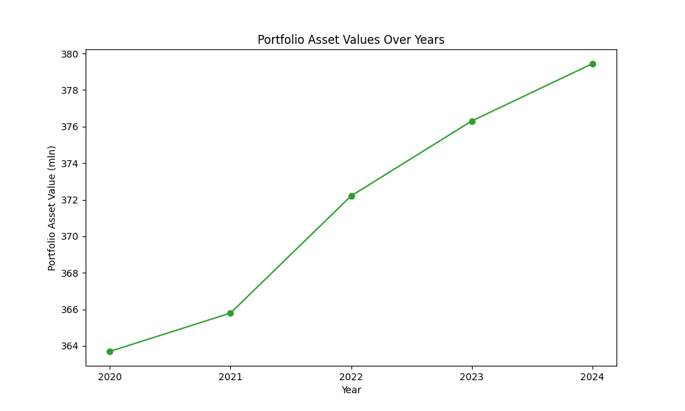
Before diving into the VaR calculation, first, we will take a short look at the general characteristics of the portfolio. You can see that the portfolio assets increased over the years, creating a portfolio of around 379 million in 2024. Of course, this entails that the absolute systematic risk will increase. The more assets in the portfolio, the more absolute risk. More interesting is the standard deviation of the return. For example, an increase in standard deviation means the returns are more volatile. A more volatile portfolio will result in a higher VaR, which means a higher systematic risk. Indicating it could be strategic to change the composition of the portfolio.
What would the VaR be for this portfolio? The VaR is a forward looking variable, therefore calculated for 2025. In this demonstration, a one-year VaR is used. The calculations determine that the VaR of this portfolio is around -27 mln. This means there is a 5% chance that the loss of this portfolio exceeds -27 mln or an approximate loss of 7%. The calculation is based on a portfolio value of 380 mln, an average mean return of 6 and a standard deviation of 6.7%.
| Year | Mean return | Standard Deviation | Absolute Value at Risk | Relative Value at Risk | |
|---|---|---|---|---|---|
| 0 | 2024 | 0.062322 | 0.067899 | -26.849045 | -0.070759 |
The difference between the absolute and relative VaR is important for portfolio strategies. Relative VaR helps to understand which sectors in the portfolio outperform others. Absolute VaR gives an insight in the absolute amount needed to hedge against potential losses.
There is some debate about the usage of the VaR: it can be misleading because it provides a certain level of safety. It therefore can increase risk taking behaviour. The VaR is a holistic method to analyse a portfolio. However, it falls short when identifying risk on a more granular level. For example a portfolio of a single trader. Such a trader could have positions that seem to aggregate to a normal distributed portfolio. If, however, the portfolio includes assets with a very small probability of a huge loss, then the VaR comes short. It does not include these large tail risk.
If you want to read more about the topic, some references:
- Holton, Glyn A. (2002). History of Value-at-Risk: 1922-1998, working paper. Boston
- Taleb, Nassim N. (1997). Dynamic Hedging. New York: John Wiley & Sons.
- Hull, John C. (2023). Risk Management and Financial Institutions, 6th Edition. Toronto.